
SionnaRTStudio: A Hands-On Wireless Digital Twin Tutorial
Published:
SionnaRTStudio is an open-source, browser-based wireless digital-twin studio built on NVIDIA Sionna RT. It turns OpenStreetMap data into an interactive 3D propagation environment where you can place transmitters and receivers, trace multipath, generate coverage maps, study mobility and handover, calculate link-level KPIs, and export channel data for further research.
This tutorial walks through the complete interface. You do not need to write a Sionna notebook to complete the workflow, but the exported data and standalone scenes can be used from Python afterward.
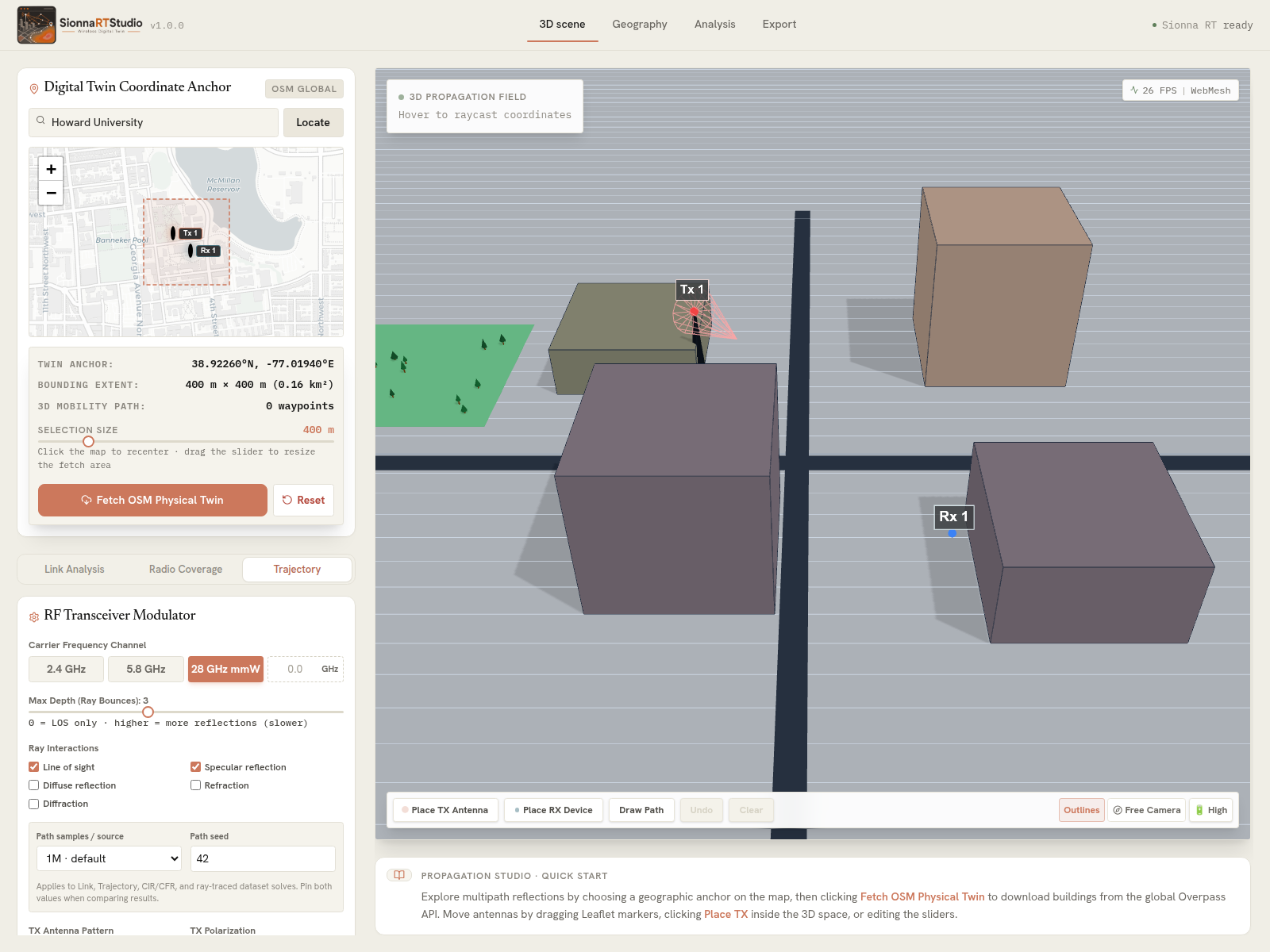 The main workspace: geographic controls on the left and the interactive Three.js digital twin on the right.
1. What the application models
SionnaRTStudio focuses on site-specific radio propagation. The backend constructs a Sionna RT/Mitsuba scene from the same building footprints displayed by the frontend and then uses GPU-accelerated ray tracing when CUDA is available.
The main study types are:
- point-to-point and all-pairs Tx/Rx link analysis;
- received-power coverage maps with multiple-transmitter best-server combining;
- receiver mobility along a user-defined trajectory;
- A3 handover analysis using per-transmitter received-power series, hysteresis, and time-to-trigger;
- channel impulse response (CIR) and channel frequency response (CFR) export;
- Shannon-capacity and MIMO channel KPIs; and
- an optional 5G NR PUSCH BER/BLER chain.
The tool is a propagation and link-research environment. Its A3 feature analyzes handover decisions, but it is not a complete gNB, UE, RRC, or core-network emulator. In 3GPP terminology, A3 is the neighbor-becomes-offset-better-than-serving measurement event used by LTE and NR mobility procedures (see 3GPP TS 36.331 and TS 38.331).
2. Requirements and installation
The easiest supported environments are Linux, macOS, or Windows through WSL2. An NVIDIA CUDA-capable GPU is strongly recommended, although SionnaRTStudio can fall back to Mitsuba’s LLVM CPU variant. Windows users should use WSL2 rather than native PowerShell or Command Prompt.
You need Python 3.11–3.13 (Python 3.14 is also supported with a NumPy version adjustment), python3-venv, and Node.js 20 or newer. If Node is missing or too old, the setup script installs a pinned project-local Node runtime automatically.
git clone https://github.com/puloktarafder/SionnaRTStudio.git
cd SionnaRTStudio
./setup.sh
./run.sh
Open http://localhost:3000. The status indicator in the upper-right corner should say Sionna RT ready (or RT-CORE ONLINE, depending on the current UI label).
The backend normally uses port 8000. If another process already owns that port, choose another one without editing the code:
SRTS_BACKEND_PORT=8011 ./run.sh
The Vite proxy reads the same variable, so the browser continues to reach the correct backend automatically. You can verify the runtime directly:
curl http://localhost:8011/api/health
Look for the active Mitsuba variant and the gpu boolean. A CUDA variant gives the best interactive performance; CPU results are equivalent but slower.
Windows with WSL2
Install Ubuntu under WSL2, keep the repository in the Linux filesystem (for example, ~/SionnaRTStudio rather than /mnt/c/...), and install the venv package before running setup:
sudo apt update
sudo apt install -y python3-venv
nvidia-smi
./setup.sh
./run.sh
Install the normal NVIDIA Windows display driver on the Windows side. Do not install a Linux NVIDIA display driver inside WSL, because WSL2 exposes the Windows driver to Linux through GPU passthrough.
3. Learn the workspace
The top navigation has four workspaces:
- 3D scene — place devices and run Link Analysis, Radio Coverage, or Trajectory studies;
- Geography — inspect the loaded physical twin and edit radio-material scattering parameters;
- Analysis — inspect link budgets, delay, capacity, MIMO, and optional PHY results; and
- Export — save the project, channel tensors, geometry, propagation reports, and a standalone Sionna RT scene.
Inside 3D scene, the three buttons above the lower-left control pane select the active solver workflow: Link Analysis, Radio Coverage, and Trajectory. The common RF controls remain consistent across these modes.
Navigate the 3D viewport
- Drag with the left mouse button to orbit, use the wheel to zoom, and drag with the right mouse button to pan.
- Hover over the canvas to inspect local coordinates.
- Outlines emphasizes building and road edges.
- Free Camera gives manual orbit control; click it to switch to Target: TX, which keeps the active transmitter centered while you inspect antenna orientation.
- High / Eco changes rendering quality and pixel density. It affects visualization performance, not the Sionna RT solver result.
- Place TX Antenna and Place RX Device arm placement mode; the next valid canvas click moves the selected device. Placement buttons do not run a solve automatically.
4. Build a physical twin
- Type a location in the Digital Twin Coordinate Anchor search box and click Locate.
- Click the map to recenter the selection.
- Drag Selection Size to choose the bounding area. Start with a small region while learning; larger scenes take longer to download and trace.
- Click Fetch OSM Physical Twin.
- Wait for the OpenStreetMap/Overpass download and 3D reconstruction to finish.
The map and 3D view use the same coordinate anchor. Buildings are extruded from their footprints, and available OSM tags help select ITU radio materials. Roads, vegetation, parks, and water provide visual geographic context.
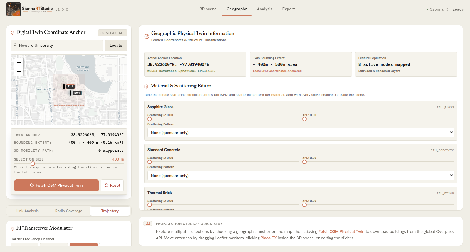 The Geography workspace reports the anchor and feature population and exposes material/scattering controls.
Use the Geography page when you need to inspect the loaded area or tune diffuse-scattering behavior. A material change affects subsequent solves, so record overrides when comparing experiments.
5. Solve a Tx-to-Rx link
Return to 3D scene and select Link Analysis.
- Place the transmitter and receiver. Drag their markers on the map, click Place TX Antenna or Place RX Device and then click in the 3D scene, or use the position controls.
- Choose the carrier frequency. The presets include 2.4 GHz, 5.8 GHz, and 28 GHz; a custom value can also be entered.
- Set Max Depth (Ray Bounces). Zero requests LOS only; higher values permit more interactions and require more computation.
- Enable the required Ray Interactions: LOS, specular reflection, diffuse reflection, refraction, diffraction, and edge diffraction where available.
- Select the path samples/source and deterministic seed. Keep both fixed for reproducible comparisons.
- Configure Tx/Rx antenna pattern, polarization, array dimensions, transmit power, height, and beam azimuth.
- Click Solve Link · Sionna RT.
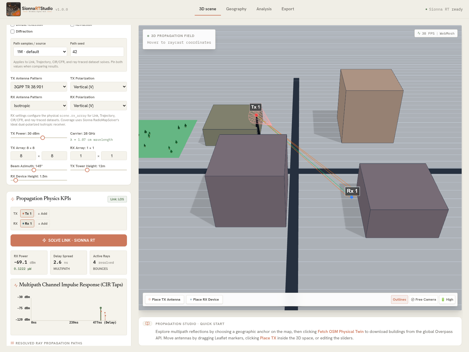 A successful solve. Colored lines are resolved propagation paths; the left panel reports link state, received power, RMS delay spread, active rays, and CIR taps.
The result panel distinguishes LOS from NLOS and reports received power in dBm, delay spread in nanoseconds, the number of resolved rays, and per-path details. With more than one transmitter or receiver, use + Add to create devices and Solve All Pairs to fill the Tx × Rx link matrix. Clicking a matrix cell focuses that pair.
Antenna, polarization, and beamforming experiments
The common RF panel supports isotropic, dipole, half-wave dipole, and 3GPP TR 38.901 element patterns; vertical, horizontal, dual, and cross polarization; configurable planar-array dimensions; and azimuth/elevation steering. The selected array and steering are applied by the backend—they are not display-only controls.
The 3GPP TR 38.901 option is an antenna element pattern. It does not by itself emulate an NR codebook, CSI feedback, or a complete beam-management procedure. SionnaRTStudio applies a steered uniform precoder, while the Analysis page reports its capacity separately from the ideal MRT bound.
For a controlled beamforming comparison:
- Keep the scene, Tx/Rx positions, carrier, interaction switches, ray budget, and seed fixed.
- Solve once with a 1 × 1 isotropic Tx.
- Increase the Tx array, select the desired element pattern, and steer toward the Rx.
- Re-solve and compare received power, path structure, and Analysis → Compute KPIs.
- Export the reproduction manifest for each configuration.
6. Generate a radio coverage map
Select Radio Coverage in the 3D-scene mode bar.
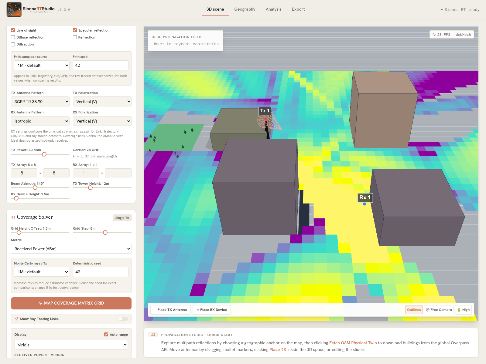 A computed received-power radio map overlaid on the 3D scene. The left panel shows the grid, Monte Carlo ray-budget, seed, and display controls used for the solve.
- Set Grid Height Offset to the receiver sampling height.
- Set Grid Step. Begin with a coarse grid, then refine only the region and resolution you need.
- Choose Received Power (dBm) or SINR (dB). SINR also exposes bandwidth and receiver noise-figure controls.
- Choose Monte Carlo rays / Tx and a deterministic seed.
- Click Map Coverage Matrix Grid.
- Under Display, select a colormap and keep Auto range enabled initially. Disable it to compare multiple runs against the same fixed scale.
When multiple transmitters exist, the coverage solver combines them using best-server selection. Show Ray-Tracing Links overlays the most recent link-solve rays; it does not replace the coverage computation.
Received power versus interference-aware SINR
| Metric | What is displayed | Important controls | Default served threshold |
|---|---|---|---|
| Received power | RSS from the strongest transmitter at each cell | Tx power, antennas, propagation interactions | −90 dBm |
| SINR | SINR of the strongest-RSS serving transmitter; every other Tx contributes interference | All power controls, channel bandwidth, receiver noise figure | 0 dB |
Best-server selection is made by received power, not by whichever transmitter happens to give the highest SINR. For SINR, the backend configures the physical thermal-noise floor from bandwidth and noise figure before reading Sionna RadioMapSolver’s SINR. This makes SINR the better view for studying overlapping multi-cell coverage, while RSS is useful for path-loss and coverage-footprint studies.
After a solve, Coverage KPIs reports the served percentage and cell-edge (p5), median (p50), and peak (p95) values. Keep the same grid, ray budget, seed, colormap range, bandwidth, and noise figure when comparing deployments. The instant JSON channel-grid proxy requires a power map because SINR is not a channel magnitude; use a received-power map or enable the genuine ray-traced CFR export.
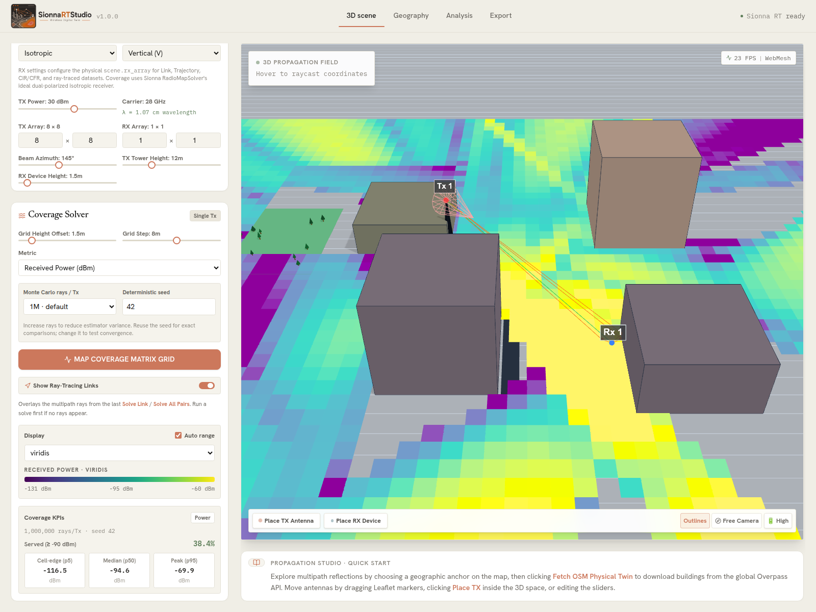 Coverage and link rays can be inspected together. Here the received-power map remains visible while Show Ray-Tracing Links overlays the resolved Tx-to-Rx paths from the latest link solve.
7. Simulate mobility and A3 handover
Select Trajectory.
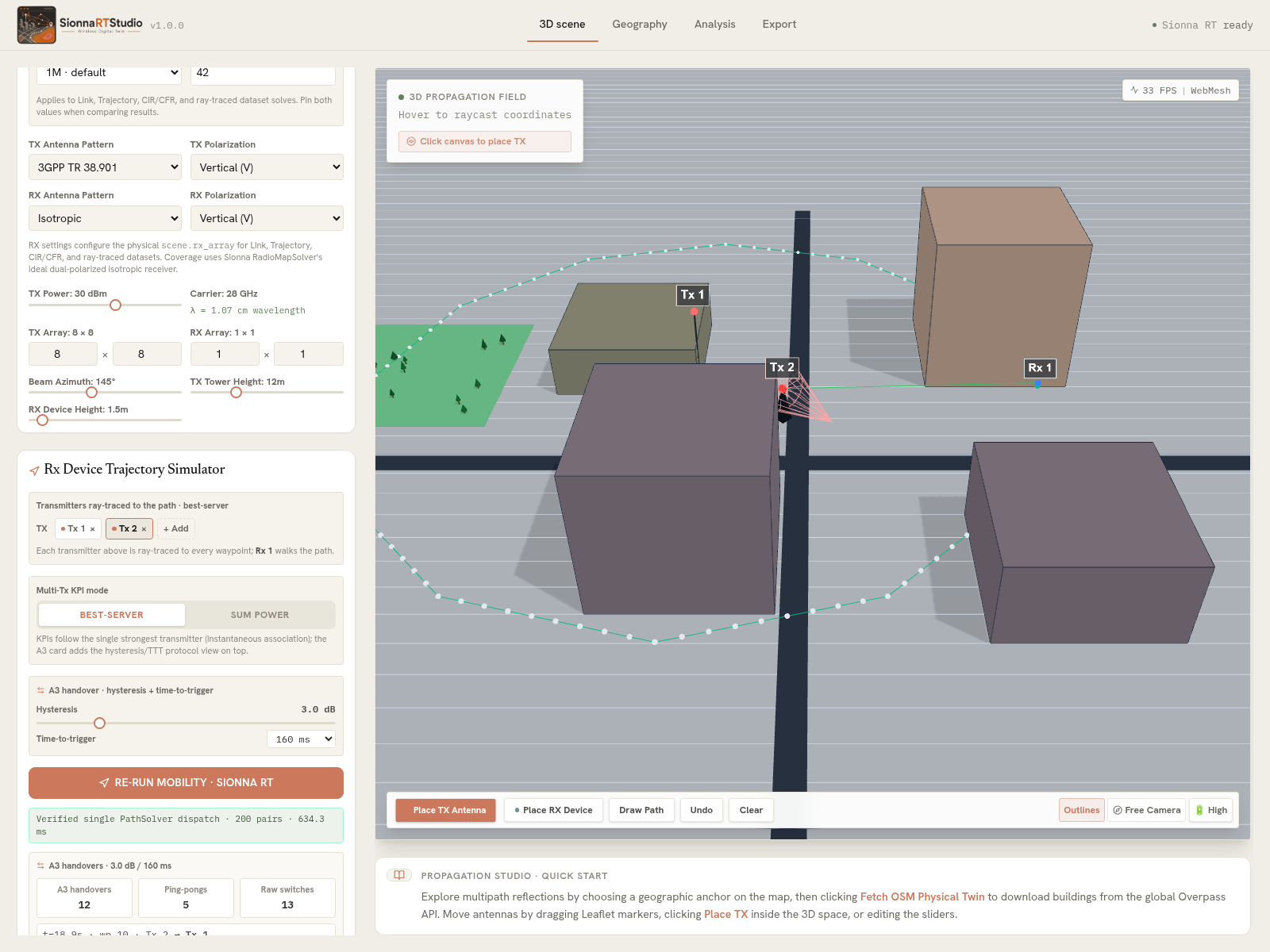 A solved 100-waypoint mobility loop with two transmitters. The panel shows best-server selection, A3 hysteresis/time-to-trigger, batched-solver telemetry, and handover statistics.
- Under Transmitters ray-traced to the path, click + Add to create at least two transmitters for a meaningful serving-cell comparison.
- Choose the KPI combination mode:
- Best-server uses the strongest transmitter at each waypoint for the headline KPIs.
- Sum power non-coherently sums incident powers while preserving the per-Tx breakdown.
- Click Draw Path, then click waypoints in the 3D scene. Use Undo or Clear to edit it. Generate Loop Path creates a quick circular example.
- For two or more transmitters, set A3 hysteresis and time-to-trigger. These values apply to the next mobility run.
- Click Run Mobility · Sionna RT. The path is defensively capped at 100 samples.
- Click Play to move the receiver through the solved steps. Drag the scrubber to inspect a particular waypoint.
At each step, the scene shows the union of rays from all transmitters, while the panel reports the serving Tx, per-Tx RSS/LOS values, received power, Doppler, and delay spread. Clicking a listed handover event jumps playback to that waypoint. The A3 summary also reports ping-pong events and the zero-hysteresis switch count for comparison.
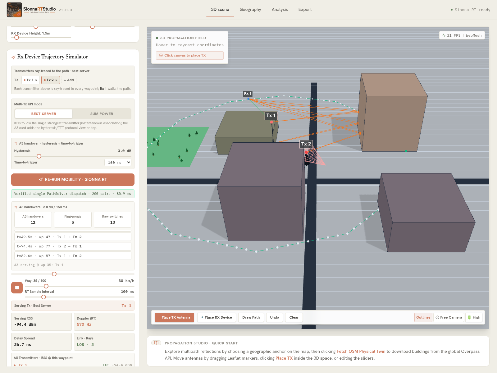 Live playback at waypoint 35 of 100. The canvas shows the complete trajectory and the per-transmitter propagation paths for the current receiver position; the panel identifies the best server and reports A3 events, RSS, Doppler, delay spread, and LOS-ray count.
All mobility transmitters currently share one antenna-array configuration because they use a common Sionna scene.tx_array.
8. Inspect channel and link-level analysis
After solving a link, open Analysis.
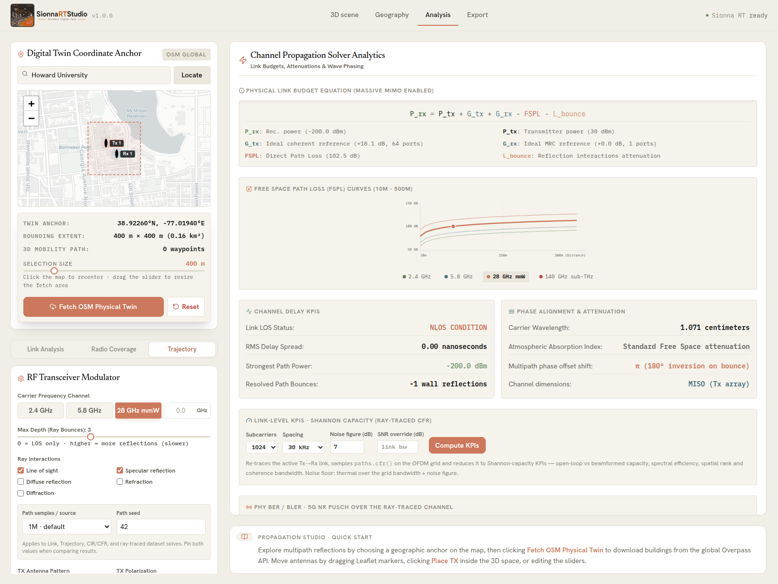 The Analysis workspace connects geometric ray tracing to link-budget, delay, MIMO, and channel-capacity interpretation.
Click Compute KPIs to re-trace the active link over the configured OFDM grid and calculate:
- open-loop MIMO capacity;
- maximum-ratio-transmission (MRT) bound;
- capacity with the applied steered uniform precoder;
- beamforming gain, spectral efficiency, and throughput;
- channel effective rank and condition number;
- coherence bandwidth; and
- link-budget effective SNR.
Before clicking, select the subcarrier count, subcarrier spacing, and receiver noise figure. Leave SNR override empty to use the physical link-budget SNR, or enter a value to compare channel capacity at a controlled operating SNR. The displayed open-loop, steered-beam, and MRT results are Shannon-capacity metrics; they are analytical bounds rather than an NR scheduler or MCS throughput prediction.
The optional Run BER Sweep sends the reciprocal uplink channel through Sionna PHY’s 5G NR PUSCH chain, including LDPC, QAM, DMRS-based estimation, and LMMSE detection. Install this large optional dependency separately:
./.venv/bin/pip install -r backend/requirements-phy.txt
The BER/BLER sweep runs as a background job. Its channel is normalized to unit mean energy, so the Eb/N0 axis emphasizes selectivity rather than path loss.
Configure MCS index, PRB allocation, Eb/N0 range, and slots per point before starting the sweep. More slots reduce Monte Carlo uncertainty but increase runtime. This full PHY result is distinct from the Shannon-capacity card: it uses coding, modulation, DMRS channel estimation, and receiver detection.
9. Save and export the experiment
Open Export when the study is complete.
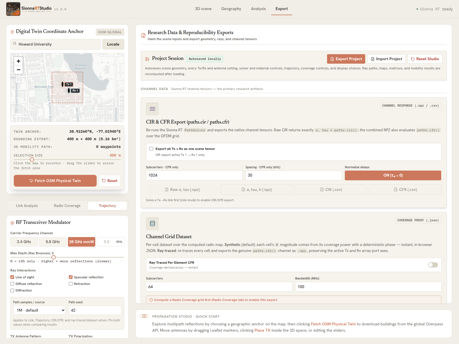 Use Project Session for editable state and the scientific export cards for channel tensors, geometry, and provenance.
Each export has a different purpose:
| Export | What it contains | Typical use |
|---|---|---|
| Project JSON | Versioned, editable scene, device, antenna, solver, material, trajectory, coverage, and display settings | Pause and resume a study, share an app configuration, or create parameter-sweep starting points. It is not a computed-results archive. |
| Experiment Reproduction Manifest | App/engine information, ENU anchor and coordinate convention, solver options and seed, material overrides, device/array definitions, a canonical input digest, and available-result summaries | Provenance, dataset cards, experiment auditing, and checking that two runs used the same inputs. |
| Raw CIR NPZ | Complex path coefficients a, path delays tau, geometric delays, carrier frequency, device metadata, and the original Tx/Rx array definitions | Delay-domain channel analysis, multipath feature extraction, delay-spread studies, and training channel or tap-set surrogate models. |
| Combined CIR/CFR NPZ | The CIR fields plus complex h_freq, baseband frequencies, and subcarrier spacing | OFDM/MIMO learning, channel estimation, CSI compression, beam or precoder selection, and frequency-selective channel emulation. |
| CIR/CFR CSV | A human-readable view of one Tx→Rx link, limited to the first antenna pair/time sample where needed | Quick plots, spreadsheet inspection, and debugging. Use NPZ—not CSV—when full MIMO tensor fidelity matters. |
| All-pairs ZIP | One exact CIR dataset per Tx × Rx pair, with a manifest mapping pairs to files | Multi-link datasets and heterogeneous device arrays. Pair-wise files avoid padding or flattening incompatible antenna dimensions. |
| Propagation CSV | One row per displayed propagation path: type, interaction order, distance, loss, received power, delay, and ENU vertices | Path classification, explainable propagation models, reflection-order statistics, and interpretable tabular features. It is not the full complex MIMO channel. |
| GeoJSON | Geographic building/feature geometry with identifiers, heights, categories, materials, and anchor metadata | GIS joins, map visualization, spatial labels, region-based dataset splitting, and geospatial ML features. |
| Wavefront OBJ | The procedural 3D digital-twin geometry, including extruded buildings and available terrain/infrastructure surfaces | Blender/CAD/Unity workflows, visualizations, geometry processing, or 3D-learning inputs. RF solver settings are stored elsewhere. |
| Coverage proxy JSON | Received power and coordinates from the coverage map plus a deterministic, synthetic per-subcarrier complex phase | Fast data-loader prototyping, RSS regression, and testing an ML pipeline before expensive channel generation. It is explicitly labeled synthetic: true and is not paths.cfr() output. |
| Ray-traced channel-grid NPZ | Genuine per-cell Sionna RT CFR h, coordinates, ray-traced LOS labels, received power, frequency grid, Tx power, and array metadata | Site-specific CSI datasets, localization, beam selection, channel estimation, and learned channel/radio-map surrogates. The h layout is [cell, Rx antenna, Tx antenna, subcarrier]. |
| Scene + load_scene.py ZIP | The exact Mitsuba scene and meshes plus a generated Sionna RT replay script and manifest | Reproduce or extend the experiment outside the web app in Python, a notebook, or a batch-compute environment. |
Computed maps and paths are intentionally regenerated after importing a project. For a reproducible research package, save the project JSON, reproduction manifest, relevant channel tensors, and geometry together.
Browser autosave, project files, and reset
Editable inputs autosave to the current browser: scene geometry, devices, solver/material settings, trajectory, coverage configuration, and display choices. Computed rays, radio maps, mobility results, KPI results, and BER sweeps are not treated as permanent state.
- Export Project creates a portable, versioned JSON file.
- Import Project validates that file and clears stale computed results so they can be regenerated.
- Reset Studio clears the editable session in the browser. Export first if the setup matters.
Browser autosave is convenient recovery, but it is not a research archive. Use the project JSON plus the reproduction manifest and scientific outputs for an experiment you intend to cite.
Load CIR/CFR data in Python
The raw export writes a (complex path coefficients) and tau (path delays). The combined NPZ also writes h_freq, the CFR over the selected OFDM grid, and frequencies, the baseband subcarrier offsets.
import numpy as np

d = np.load("sionna_rt_studio_cir_cfr.npz")
a = d["a"]
tau = d["tau"]
h = d["h_freq"]
frequencies = d["frequencies"]

print("CIR coefficients:", a.shape)
print("Path delays:", tau.shape)
print("CFR:", h.shape)
NPZ preserves device and antenna axes. CSV is intentionally limited to one Tx→Rx link because flattening a multi-device MIMO tensor would be ambiguous. If device array sizes differ, use Export all-pairs ZIP; it preserves each pair’s actual array configuration instead of padding incompatible tensors.
Choosing exports for an AI/ML dataset
Choose the label and representation from the scientific question rather than exporting every format indiscriminately:
- For coverage or RSS prediction, combine coordinates and received-power labels with GeoJSON scene features. The coverage proxy JSON is useful here, but its generated complex phases must not be presented as physical CSI.
- For CSI prediction, channel estimation, localization, or beam selection, use the ray-traced channel-grid NPZ or combined CIR/CFR NPZ. Preserve the complex real/imaginary components and antenna/subcarrier axes unless the model intentionally consumes a derived representation.
- For multipath or explainable propagation research, use raw CIR NPZ together with Propagation CSV. Delays, interaction types, orders, and vertices provide interpretable features that a frequency-domain tensor alone does not expose.
- For geometry-aware or multimodal learning, pair GeoJSON or OBJ with channel tensors and the reproduction manifest. Use the ENU anchor and feature identifiers to keep geometry and radio labels aligned.
- For multi-cell or multi-device studies, use the all-pairs ZIP and keep the Tx/Rx identifiers from its manifest. Do not silently concatenate links with different array shapes.
Nearby radio-map cells are strongly correlated, so a random cell-level train/test split can leak nearly identical geometry into both sets. Prefer splits by spatial region, trajectory, transmitter, or entire scene. Keep carrier frequency, array pattern/polarization, solver interactions, depth, ray budget, seed, coordinate convention, and any normalization procedure beside every dataset release. Path enumeration order can vary between runs; sort paths by delay or use a permutation-invariant representation when path order is not itself meaningful.
The full ray-traced grid is much more expensive than the proxy and is capped at 16,384 cells. Recompute the coverage map with a coarser grid if the export exceeds that limit. Never mix proxy samples and genuine ray-traced CFR samples without retaining their synthetic/dataset-kind labels.
Run the standalone exported scene
Scene + load_scene.py (.zip) is a portable reconstruction of the actual scene sent to Sionna RT—not a screenshot or a generic OBJ conversion. Its contents are:
scene.xml          Mitsuba scene and ITU radio-material BSDF assignments
meshes/*.ply       Ground and building meshes referenced by relative paths
load_scene.py      Generated Sionna RT experiment/replay code
manifest.json      Machine-readable settings, devices, arrays, and file mapping
README.md          Bundle-specific usage and fidelity notes
scene.xml describes geometry and Mitsuba-side materials. However, a standalone XML file cannot retain all Sionna-side experiment state. The generated load_scene.py therefore restores the carrier frequency, material overrides, PlanarArray definitions, every Tx/Rx position, transmit power and steering, and the selected PathSolver interaction switches. It then calls paths.cir() and paths.cfr() using the exported OFDM settings. This is the bridge between the browser experiment and an ordinary Sionna RT Python workflow.
Extract the ZIP into its own directory, create an environment with Sionna RT, and run it without SionnaRTStudio:
pip install sionna-rt
python load_scene.py
For a scene whose devices use compatible array sizes, the script writes one dense cir.npz. Sionna RT uses one scene-wide Tx array and one scene-wide Rx array, so heterogeneous device arrays cannot be represented honestly in a single dense tensor. In that case, the script solves exact array-compatible groups into channels/*.npz; manifest.json maps every group and ensures that all Tx × Rx pairs remain covered without padding or substituting arrays.
Use it from a Jupyter notebook
The most faithful notebook workflow is to execute the generated replay script from the extracted directory:
%cd /path/to/extracted/sionna_rt_studio_scene
%run load_scene.py

import numpy as np

d = np.load("cir.npz")  # for a uniform-array export
print(d.files)
print("a:", d["a"].shape, "tau:", d["tau"].shape)
if "h_freq" in d:
    print("h_freq:", d["h_freq"].shape)
For a heterogeneous-array export, read manifest.json and load the files listed under its array groups from channels/ instead of assuming cir.npz exists. Running %run load_scene.py performs the complete reconstruction and leaves the generated Python objects available for further notebook analysis.
If only geometry inspection is needed, the scene can also be loaded directly:
from sionna.rt import load_scene

scene = load_scene("scene.xml")
Import sionna.rt before loading the XML so its radio-material plugin is registered. Directly loading scene.xml restores the geometry and material BSDFs, but it does not by itself recreate the exported carrier, arrays, devices, steering, or solver settings. Use load_scene.py for exact replay, or copy its generated setup into notebook cells and adapt it—for example, to change the Tx/Rx sweep, compute a new OFDM grid, add a RadioMapSolver, or generate a larger research dataset on a compute server.
All exported positions use local ENU metres: x east, y north, z up, with ground at z = 0. Preserve the anchor in manifest.json when joining channel samples back to geographic data. Transmit power is retained for link budgets and radio-map work; it does not directly rescale the CIR/CFR coefficients returned by Sionna RT.
10. Recommended reproducible study workflow
- Load a small OSM area and export the project immediately as the baseline.
- Place devices and set carrier, arrays, patterns, polarization, interactions, ray budget, and seed.
- Solve one link and inspect the resolved paths before launching a larger coverage or mobility job.
- For coverage comparisons, pin grid size, height, metric, bandwidth/noise figure, ray budget, seed, and color scale.
- For mobility comparisons, pin the trajectory, speed, sample interval, combination mode, hysteresis, and time-to-trigger.
- Export native CIR/CFR and the reproduction manifest; include GeoJSON or OBJ when scene geometry must be preserved independently.
- Change one experimental variable at a time and keep each project’s JSON beside its outputs.
Which results unlock which exports?
| First produce | Then you can use |
|---|---|
| Loaded building geometry | Standalone scene ZIP, manifest, OBJ, GeoJSON |
| Solved Tx→Rx link | CIR/CFR exports, propagation CSV, link-level KPIs |
| Solved all-pairs or active link | Ray overlay on the coverage view |
| Computed power coverage map | Coverage proxy JSON or ray-traced channel-grid NPZ |
| Installed optional Sionna PHY package | 5G NR PUSCH BER/BLER sweep |
11. Quick click reference
| Goal | Where to go | Click |
|---|---|---|
| Download a real scene | 3D scene → map | Fetch OSM Physical Twin |
| Move a device in 3D | 3D scene | Place TX Antenna or Place RX Device |
| Trace one radio link | 3D scene → Link Analysis | Solve Link · Sionna RT |
| Compare every device pair | 3D scene → Link Analysis | Solve All Pairs |
| Compute a coverage heatmap | 3D scene → Radio Coverage | Map Coverage Matrix Grid |
| Compare interference-aware coverage | 3D scene → Radio Coverage | Select SINR (dB), then map coverage |
| Draw receiver mobility | 3D scene → Trajectory | Draw Path |
| Solve and replay mobility | 3D scene → Trajectory | Run Mobility · Sionna RT, then Play |
| Calculate capacity KPIs | Analysis | Compute KPIs |
| Run the optional NR PHY chain | Analysis | Run BER Sweep |
| Save editable work | Export | Export Project |
| Reproduce outside the app | Export | Scene + load_scene.py (.zip) |
12. Troubleshooting
The backend badge is offline. Check the terminal that launched ./run.sh, confirm the selected Python can import sionna and fastapi, and query /api/health directly.
Port 8000 is occupied. Start with SRTS_BACKEND_PORT=8011 ./run.sh; do not terminate an unrelated service merely to reclaim the default port.
CPU startup reports a missing LLVM library. On Ubuntu without CUDA, install it with sudo apt install llvm-runtime.
A solve takes too long. Reduce the geographic extent, max depth, path samples, coverage ray budget, or coverage-grid resolution. Confirm /api/health reports "gpu": true if a supported NVIDIA GPU should be available.
No rays appear. Confirm that a Tx and Rx are placed, the backend is online, at least one interaction type is enabled, and a solve has completed. Geometry can block LOS, so enable the relevant reflection/diffraction mechanisms when studying NLOS links.
An export button is disabled. Generate its prerequisite first using the table above. In particular, CIR/CFR needs a solved link, and channel-grid export needs a coverage map.
SINR controls or values look different from power coverage. Bandwidth and noise figure apply only to SINR. Manual dBm display limits are intended for power maps; use the metric-aware auto range for SINR.
Next steps
Start with the preloaded demo scene and one link solve, then move to a small familiar OpenStreetMap region. Once the result is stable, add coverage, multiple transmitters, and a trajectory. Change one parameter at a time and pin random seeds when comparing antenna patterns, material settings, or solver budgets.
The source code, installation scripts, and detailed technical notes are available in the SionnaRTStudio GitHub repository.